

Attention from First Principles - 4
Linear Attention and the Memory Wall

The first three posts built up a complete picture of modern attention — from the raw mechanics of scaled dot-product attention, through multi-head attention and causal masking, to Grouped Query Attention and Multi Head Latent Attention.
you can refer to the previous articles here (highly recommended if you have not already read):
Parameter-sharing tricks of GQA (Grouped Query Attention) and MLA (Muti-Head Latent Attention) made attention cheaper to run.
But none of it changed the fundamental cost structure.
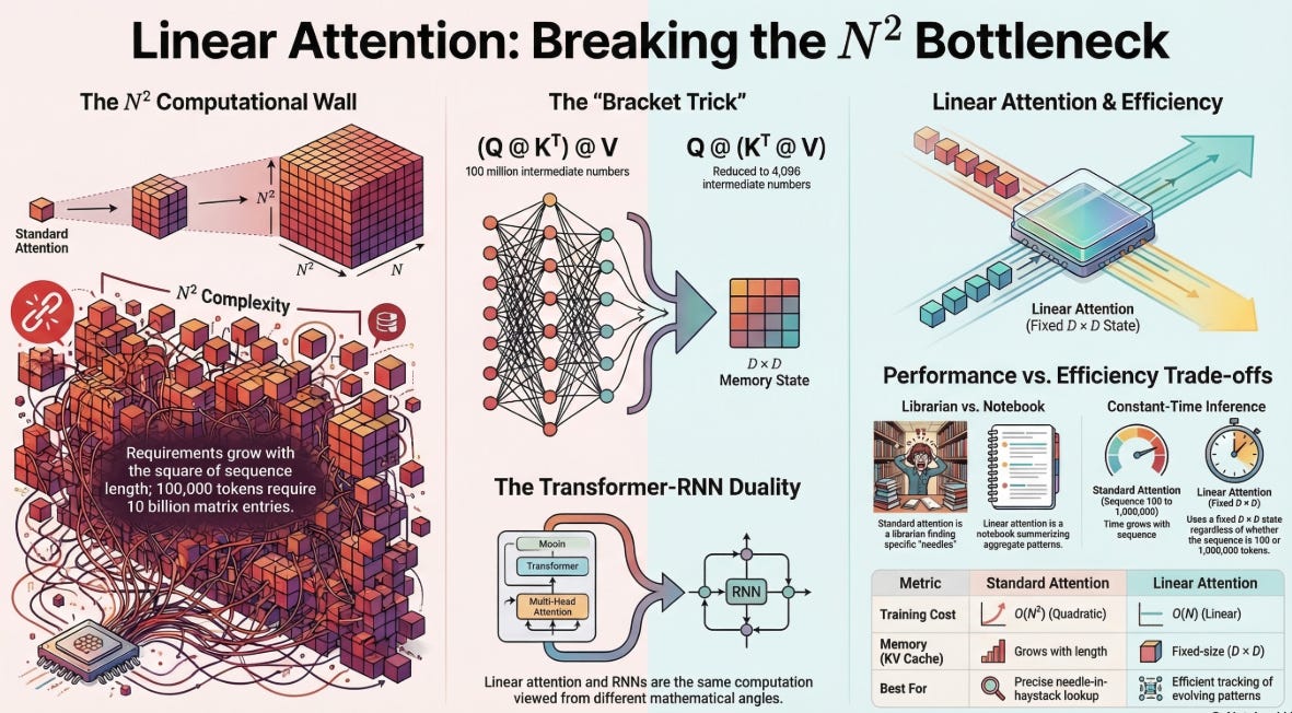
The attention matrix is N×N, where N is your sequence length. At 512 tokens that’s fine. At 4,000 tokens — a long document — you’re at 16 million entries. At 100,000 tokens, you’re at 10 billion. The memory and compute requirements don’t grow with your sequence length, they grow with its square.
GQA and MLA reduce the size of the K and V projections. Flash Attention tiles the computation to fit in fast memory. These are real gains. But you’re still computing an N×N matrix. The wall is still there.
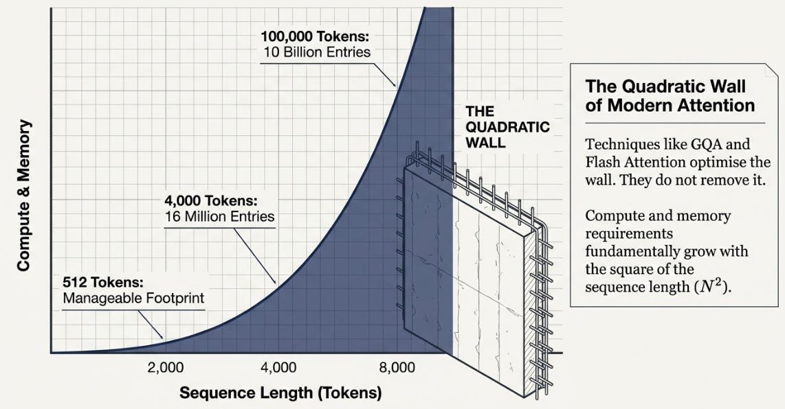
Linear Attention doesn’t optimize the wall. It removes it — by asking whether you need that N×N matrix at all.
And in answering that question, something unexpected turns up: transformers and RNNs, long treated as competing ideas, turn out to be the same thing looked at from different angles. (I will cover how as we move along in this post so keep reading!!)
The Bracket Trick
Standard attention computes:
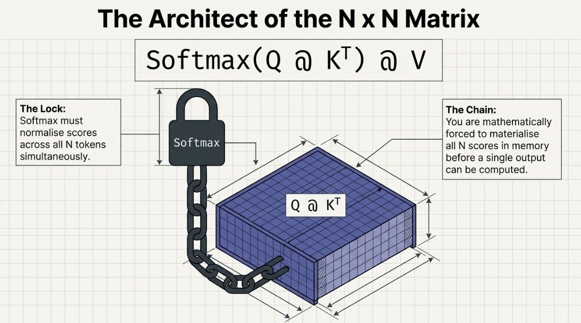
Output = softmax(Q @ K^T) @ VThe bottleneck is Q @ K^T. Q has shape (N, D) and K has shape (N, D), so their product is (N, N) — one score for every token pair. That’s the matrix that kills you at long sequence lengths.
Now, Softmax is the reason standard attention has to form this matrix. It normalizes across all N scores for each token — which means you need all N scores in memory at once before you can compute a single output. There’s no way around it.
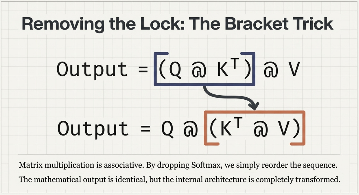
But what if you dropped the Softmax? The operation becomes:
Output = (Q @ K^T) @ VAnd matrix multiplication is associative. You can reorder the brackets:
Output = Q @ (K^T @ V)The result is mathematically identical. But the computation is radically different.
Concrete example. Say N = 10,000 tokens and D = 64:
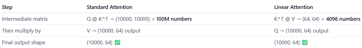
Same output shape. Same result. One of them materializes 100 million numbers in the middle. The other materializes 4,096.
S = K^T @ V is a fixed-size compressed summary of the entire sequence. It doesn’t grow with N — ever.
The cost of dropping Softmax is real though — we’ll come to that shortly.
What You Lose Without Softmax
Softmax does two things. It makes attention scores sum to one, and it sharpens them — pushing high scores higher and low scores lower. The result is that each output token attends strongly to a small number of relevant past tokens and mostly ignores the rest.
Without Softmax, you lose both properties. The D×D state S is a flat accumulation — every past token contributes to it, weighted only by raw dot product magnitude. Ask S about the main character and it returns a blend of every character it has seen, not the one most relevant to your query.
But the trade-off runs deeper than just “sharp vs. blurry.”
What standard attention is good at: Finding a specific needle in a haystack. If the answer to a question depends on one precise earlier token — a name, a number, a rare fact — softmax attention will find it. The N×N matrix exists precisely to enable that kind of surgical lookup.
What linear attention is good at: Tracking patterns that accumulate over time. If the answer depends on the aggregate of many past tokens — the general topic, the overall sentiment, the statistical tendency — S handles that well. It’s essentially a running average of the sequence’s key-value associations.
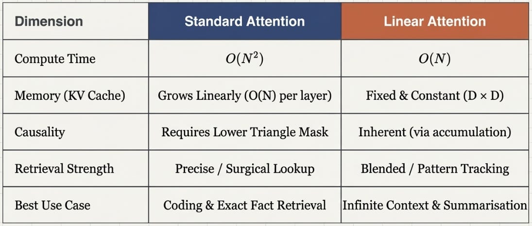
The memory trade-off: Standard attention at inference time must store every past K and V vector — the KV cache grows linearly with sequence length. At 100k tokens with D=4096, that’s gigabytes per layer. Linear attention stores only S — a fixed D×D matrix, always the same size regardless of sequence length.
The compute trade-off: Standard attention at training time is O(N²). Linear attention is O(N). For short sequences the difference is small. For sequences above ~8k tokens, it becomes the deciding factor.
Neither is strictly better. Standard attention has sharper recall. Linear attention has bounded memory and linear cost. The right choice depends on whether your task needs precise lookup or efficient accumulation.
A Quick Detour: Outer Products
You’re already familiar with the dot product — multiply two vectors element-wise and sum. The result is a single number that measures similarity.
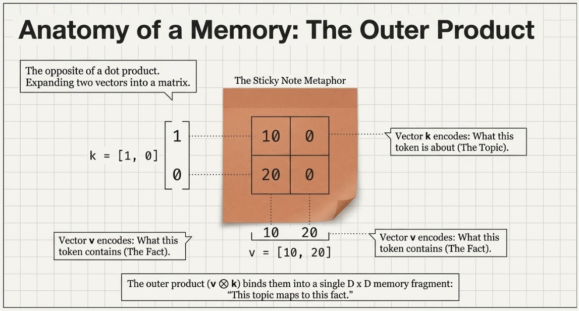
The outer product is the opposite move. Instead of collapsing two vectors into a scalar, you expand them into a matrix — every element of the first vector paired with every element of the second:
v = [10, 20]      k = [1, 0]

v ⊗ k = [[10×1, 10×0],   =  [[10,  0],
[20×1, 20×0]] [20, 0]]Shape-wise: a vector of size D times a vector of size D gives a (D, D) matrix.
The intuition: the outer product associates every dimension of v with every dimension of k. If k encodes “what this token is about” and v encodes “what this token contains”, then
v ⊗ kis a small memory fragment: “this topic maps to this fact.”
Building the Memory State
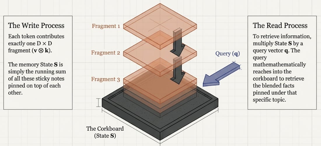
Each token contributes one outer product — a (D, D) fragment that encodes its key-value association. The state S is just the running sum of all these fragments:
S_0 = zeros(D, D)
S_1 = S_0 + v_1 ⊗ k_1
S_2 = S_1 + v_2 ⊗ k_2
S_3 = S_2 + v_3 ⊗ k_3
Concrete example. Three tokens, D=2:
Token 1: k=[1,0], v=[10,20]    →  fragment: [[10, 0], [20, 0]]
Token 2: k=[0,1], v=[30,40]    →  fragment: [[ 0,30], [ 0,40]]
Token 3: k=[1,1], v=[50,60]    →  fragment: [[50,50], [60,60]]

S after token 1: [[10,  0], [20,  0]]
S after token 2: [[10, 30], [20, 40]]
S after token 3: [[60, 80], [80,100]]
To retrieve — say after token 2, with query q=[1,0]:
S_2 @ q = [[10,30],[20,40]] @ [1,0] = [10, 20]The query [1,0] picks out the first column of S — which is exactly what token 1 wrote there.
Quick Detour: Matrix × Vector Multiplication
A matrix times a vector works row by row. Each row of the matrix takes a dot product with the vector, producing one number in the output.
S = [[10, 30],      q = [1,
     [20, 40]]           0]

output[0] = (10×1) + (30×0) = 10
output[1] = (20×1) + (40×0) = 20

result = [10, 20]
That’s it. Each row of S “asks” the query: how much of me do you want? The dot product is the answer.
Now watch what q is doing here. q = [1, 0] is selecting the first column of S. If q were [0, 1], it would select the second column. And [0.5, 0.5] would give an equal mix of both.
So,
S @ qis a lookup — not a search through past tokens, but a read from a compressed memory, guided by the query.
The Surprising Link to Recurrence
Look at the update pattern again:
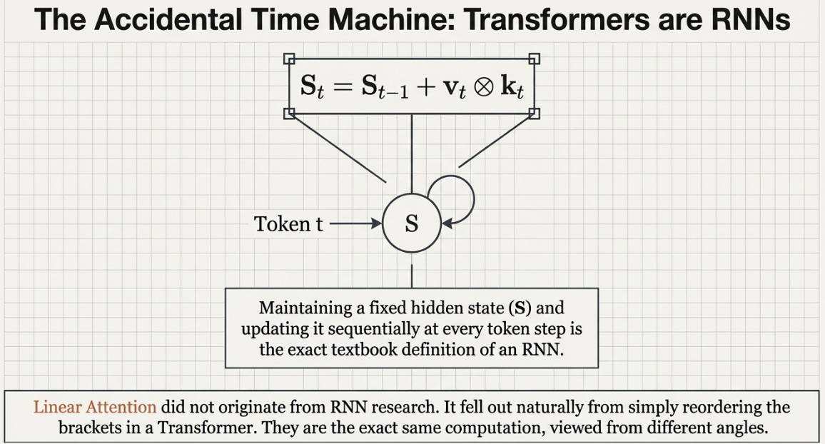
S_t = S_{t-1} + v_t ⊗ k_t
o_t = S_t @ q_t
This is a recurrent computation. S is a hidden state. It gets updated at every token. The output is read from it at every step. If you showed this to someone familiar with RNNs but not transformers, they’d recognize it immediately — it’s just an RNN with a matrix hidden state instead of a vector.
The surprise is that this didn’t come from RNN research. It fell out naturally from asking a simple question: what if we just reordered the brackets in the attention formula?
Linear Attention and RNNs aren’t two different ideas. They’re the same computation written in different order.
But there’s a subtlety here. The parallel computation Q @ (K^T @ V) builds one global S from the entire sequence — every token sees the full context, including future tokens. That’s not causal.
In standard attention, causality comes from masking the N×N matrix with a lower triangle. But there is no N×N matrix in linear attention — S has already collapsed the sequence dimension into D×D.
The recurrent form gives you causality for free. At step t, S contains only tokens 0 through t — future tokens haven’t been added yet. No masking needed.
The practical consequence is powerful: you train in parallel mode (fast, GPU-friendly), and deploy in recurrent mode (constant memory, one token at a time). Same model, same weights, two execution strategies.
Proving the Equivalence
Let’s verify with concrete numbers that both modes produce identical results. Same three tokens, D=2:
K = [[1,0],    V = [[10,20],    Q = [[1,0],
     [0,1],         [30,40],         [0,1],
     [1,1]]         [50,60]]         [1,1]]
Recurrent mode — build S token by token, query at each step:
S_0 = [[0,0],[0,0]]

Step 1:  S_1 = S_0 + v_1 ⊗ k_1 = [[10, 0],[20, 0]]
         o_1 = S_1 @ q_1 = [[10,0],[20,0]] @ [1,0] = [10, 20]

Step 2:  S_2 = S_1 + v_2 ⊗ k_2 = [[10,30],[20,40]]
         o_2 = S_2 @ q_2 = [[10,30],[20,40]] @ [0,1] = [30, 40]

Step 3:  S_3 = S_2 + v_3 ⊗ k_3 = [[60,80],[80,100]]
         o_3 = S_3 @ q_3 = [[60,80],[80,100]] @ [1,1] = [140, 180]
Recurrent output: [[10,20], [30,40], [140,180]]
Parallel mode — but we need causality. Apply a lower-triangular mask to the attention scores:
Scores = Q @ K^T = [[1,0,1],
                     [0,1,1],
                     [1,1,2]]

Causal mask:        [[1,0,0],
                     [1,1,0],
                     [1,1,1]]

Masked scores:      [[1,0,0],
                     [0,1,0],
                     [1,1,2]]

Output = masked scores @ V:

  o_1 = 1×[10,20] + 0×[30,40] + 0×[50,60] = [10, 20]
  o_2 = 0×[10,20] + 1×[30,40] + 0×[50,60] = [30, 40]
  o_3 = 1×[10,20] + 1×[30,40] + 2×[50,60] = [140, 180]
Parallel output: [[10,20], [30,40], [140,180]]
Identical. ✅
Linear Attention in Code
Let’s implement both modes — recurrent and parallel — so you can see the mechanics clearly and verify they match.
First, the setup. Three tokens, embedding dimension D=2:
import torch

K = torch.tensor([[1., 0.], [0., 1.], [1., 1.]])
V = torch.tensor([[10., 20.], [30., 40.], [50., 60.]])
Q = torch.tensor([[1., 0.], [0., 1.], [1., 1.]])
Recurrent mode. This is the RNN form — loop through tokens, updating S at each step:
S = torch.zeros(2, 2)
out_recurrent = []

for t in range(3):
    # Write: add new key-value association to memory
    S = S + V[t].unsqueeze(1) @ K[t].unsqueeze(0)
    # Read: query the current state
    out_recurrent.append(S @ Q[t])

out_recurrent = torch.stack(out_recurrent)
The V[t].unsqueeze(1) @ K[t].unsqueeze(0) line is the outer product — it reshapes v from (D,) to (D,1) and k from (D,) to (1,D), then multiplies to get a (D,D) fragment. Each fragment is one token’s contribution to memory.
Parallel mode. No loop — compute everything in bulk using three operations:
# Step 1: All outer products at once
outer_products = V.unsqueeze(2) * K.unsqueeze(1)   # (3, 2, 2)

# Step 2: Running sum gives S at each timestep
S_all = torch.cumsum(outer_products, dim=0)         # (3, 2, 2)

# Step 3: Query each state with its corresponding Q
out_parallel = torch.einsum(’tde,te->td’, S_all, Q) # (3, 2)
Step 1 computes all three outer products simultaneously — V.unsqueeze(2) gives shape (3,2,1) and K.unsqueeze(1) gives (3,1,2), broadcasting produces (3,2,2). Step 2 runs a cumulative sum along the token dimension, so S_all[t] contains the accumulated state after seeing tokens 0 through t — this is where causality comes from. Step 3 uses einsum to query each state — 'tde,te->td' means “for each timestep t, multiply the (D,D) state by the (D,) query vector.”
Verification:
print(”Recurrent:\n“, out_recurrent)
print(”Parallel:\n“, out_parallel)
print(”Match?”, torch.allclose(out_recurrent, out_parallel))

Recurrent:
 tensor([[ 10.,  20.],
        [ 30.,  40.],
        [140., 180.]])
Parallel:
 tensor([[ 10.,  20.],
        [ 30.,  40.],
        [140., 180.]])
Match? True
Same result. The recurrent mode loops through one token at a time, maintaining a single (D,D) state. The parallel mode computes the same thing in three bulk tensor operations with no loop. Two execution strategies, identical output.
From Toy Example to Training Code
The core logic doesn’t change — we just add the dimensions real training needs. Here’s a complete nn.Module you can actually train with:
import torch
import torch.nn as nn

class LinearAttention(nn.Module):
    def __init__(self, d_model, n_heads):
        super().__init__()
        assert d_model % n_heads == 0
        self.n_heads = n_heads
        self.head_dim = d_model // n_heads

        self.q_proj = nn.Linear(d_model, d_model, bias=False)
        self.k_proj = nn.Linear(d_model, d_model, bias=False)
        self.v_proj = nn.Linear(d_model, d_model, bias=False)
        self.o_proj = nn.Linear(d_model, d_model, bias=False)
        self.norm = nn.GroupNorm(n_heads, d_model)

    def forward(self, x):
        B, N, _ = x.shape
        H, D = self.n_heads, self.head_dim

        # Project input to Q, K, V and split into heads
        q = self.q_proj(x).view(B, N, H, D)
        k = self.k_proj(x).view(B, N, H, D)
        v = self.v_proj(x).view(B, N, H, D)

        # Step 1: All outer products at once
        # (B, N, H, D, 1) * (B, N, H, 1, D) -> (B, N, H, D, D)
        outer = v.unsqueeze(-1) * k.unsqueeze(-2)

        # Step 2: Cumulative sum along sequence dimension -> causal states
        S_all = torch.cumsum(outer, dim=1)

        # Step 3: Query each state
        # For each (B, N, H): multiply (D, D) state by (D,) query
        out = torch.einsum(’bnhde,bnhe->bnhd’, S_all, q)

        # Merge heads, normalize, project
        out = out.reshape(B, N, H * D)
        out = self.norm(out.transpose(-1, -2)).transpose(-1, -2)
        return self.o_proj(out)
Let’s verify it runs:
model = LinearAttention(d_model=64, n_heads=4)
x = torch.randn(2, 128, 64)   # batch=2, seq_len=128, d_model=64
out = model(x)
print(out.shape)               # torch.Size([2, 128, 64])
The shapes tell the story. The input is (B, N, d_model). It flows through as (B, N, H, D) internally — one state matrix per head per batch item. The cumsum along dim=1 builds the causal running state, exactly as in our toy example. GroupNorm prevents the accumulated state from exploding in magnitude, and the output projection merges the heads back to d_model.
The only new concept here is unsqueeze(-1) and unsqueeze(-2) — these are the same outer product trick from before, just operating on the last two dimensions instead of the first two, because of our batch and head dimension.
Mental Models to Take With You
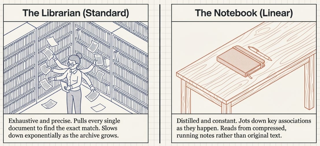
Standard Attention is a librarian. Every time you ask a question, she walks through the entire archive, pulls out every document, scores each one for relevance, and hands you a weighted blend of the best matches. Thorough, precise — and increasingly slow as the archive grows.
Linear Attention is a notebook. As you read each new page, you jot down the key associations — “main character → Harry”, “setting → Hogwarts”. When someone asks a question, you don’t go back to the original pages. You just look at your notes. Fast, constant-time lookup — but your notes are a compressed summary, not a perfect record.
The recurrent view is reading left to right. You process one word at a time, updating your notebook as you go. At any point, your notes reflect everything you’ve read so far and nothing you haven’t. Causality isn’t enforced — it’s just how reading works.
The parallel view is reading the whole page at once. You take in all the words simultaneously and build the same notebook. Faster on hardware that can process things in parallel — but now you need to be careful not to let later words leak into earlier notes.
Both views produce the same notebook. That’s the key insight. Whether you read left-to-right or all-at-once, the final state S is identical. One is natural for inference (one token at a time), the other is natural for training (everything at once on a GPU).
The outer product is a sticky note. It takes a topic (k) and a fact (v) and binds them together into a small card. “Main character → Harry” becomes a D×D grid where the topic dimensions point to the fact dimensions. Each token produces one sticky note. S is the corkboard where all the sticky notes are pinned on top of each other.
Querying S is pulling on one thread. When you multiply S by a query q, you’re asking “what facts are associated with this topic?” The matrix multiplication reaches into the corkboard and retrieves whatever was pinned under that topic — blended across all the sticky notes that overlap there.
Where This Leaves Us
Linear Attention replaces the N×N attention matrix with a fixed D×D state that never grows. The cost drops from quadratic to linear. The KV cache disappears entirely — replaced by a compact memory matrix that works the same whether your sequence is a hundred tokens or a million.
The price is precision. Standard attention can pinpoint the one token that matters in a sea of thousands. Linear attention returns a blended average from its compressed memory. For tasks that need sharp, exact retrieval over long distances, that’s a real loss.
But here’s what makes this more than an academic trade-off: the D×D state S is writeable. Right now we’re just blindly accumulating — every token adds to S, nothing is ever removed. The state fills up with stale associations and has no mechanism to say “this fact is outdated, forget it.”
Which raises a natural question. What if S could selectively forget? What if, at every token, the model could decide — based on what it’s currently reading — how much of its old memory to keep and how strongly to write the new information?
That’s exactly what Gated Linear Attention does (Yang et al., 2023). And layered on top of that, the Delta Rule (Yang et al., 2024) adds something even sharper: before writing a new fact, check whether S already knows it, and only write the correction. But that’s the next post.
Stay Tuned!!
References
Katharopoulos et al., “Transformers are RNNs: Fast Autoregressive Transformers with Linear Attention” (2020) — the bracket trick and the RNN equivalence