

Attention from First Principles - 6
DeltaNet: Error-Driven Memory Updates for Linear Attention

You write in your notes:
“The culprit is Harry.”
A few pages later, the story confirms it again.
So you write it again.
And again.
Then the story changes.
It’s not Harry. It’s Hermione.
Now your notes contain both — the old belief and the new one.
But you don’t rewrite the entire page.
You just fix the mistake.
So the question is:
Why should a model rewrite what it already knows, instead of just correcting what it gets wrong?
Part 5 gave the linear attention state two controls — a forget gate to fade old memory and an input gate to modulate new writes. GLA was a big step forward from blind accumulation. But there’s something slightly wasteful about it.
When GLA writes a new key-value pair into S, it doesn’t check what’s already there. If S already knows that the main character is Harry, and the current token says the main character is Harry again, GLA writes the full association a second time. Worse, if the answer has changed — say the main character is now Hermione — GLA writes the new fact on top of the old one, hoping the forget gate decayed the stale entry enough. It never explicitly corrects the error.
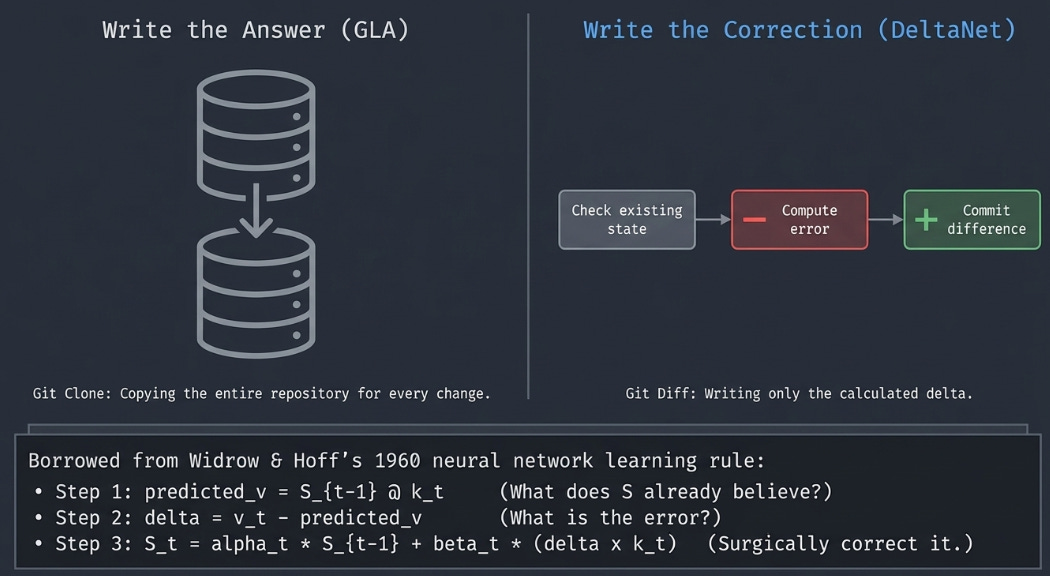
The Delta Rule fixes this with a simple idea borrowed from classical neural network training: before writing, check what S already believes, compute the error, and write only the correction.
The Delta Rule: Write the Correction, Not the Answer
GLA’s update writes the full value into memory:
S_t = α_t ⊙ S_{t-1} + β_t · (v_t ⊗ k_t)DeltaNet adds one step before writing. It queries S with the current key to see what S already predicts for that key:
predicted_v = S_{t-1} @ k_tThen it computes the error — the gap between what S believes and what the actual value is:
delta = v_t - predicted_vAnd writes only that correction:
S_t = α_t ⊙ S_{t-1} + β_t · (delta ⊗ k_t)If S already has the right answer, predicted_v ≈ v_t, the delta is near zero, and S is barely touched. If S has stale or wrong information, the delta is large, and the write surgically corrects it.
This is where the name comes from. The delta rule was proposed by Widrow and Hoff in 1960 as one of the earliest neural network learning rules — adjust weights in proportion to the prediction error. DeltaNet applies that same principle to the recurrent state, sixty years later.
GLA vs DeltaNet: A Side-by-Side
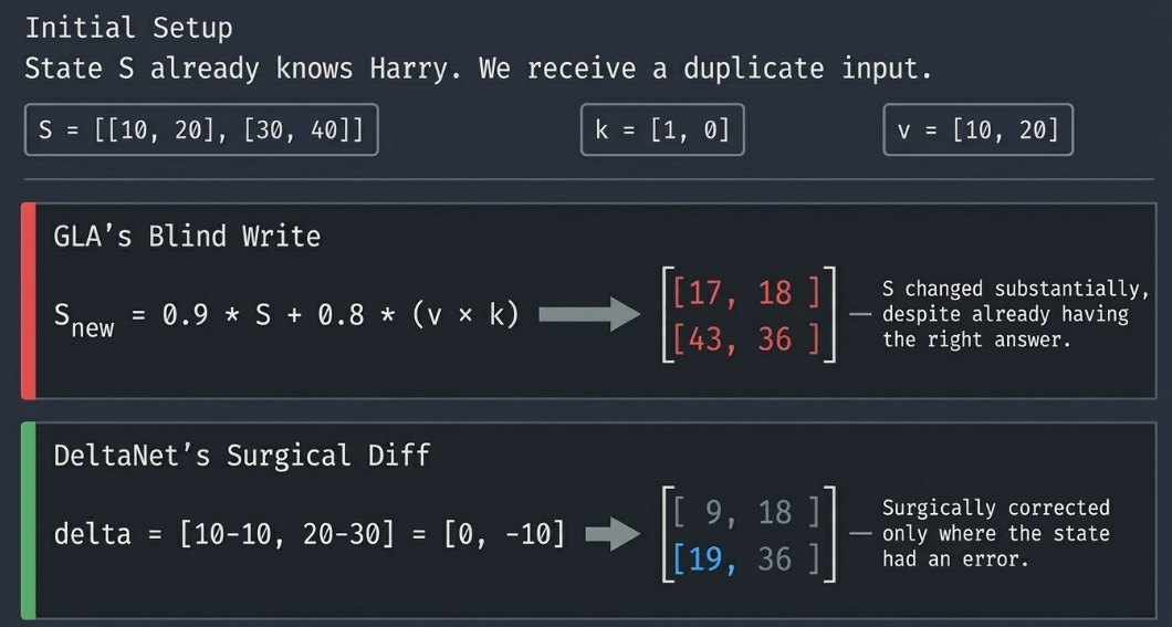
Start with a state S that already knows “main character → Harry”:
S = [[10, 20],
     [30, 40]]

k = [1, 0]     ← key for "main character"
v = [10, 20]   ← value for "Harry" (same fact, repeated)
α = [0.9, 0.9]
β = [0.8, 0.8]
GLA writes the full value blindly:
outer = v ⊗ k = [[10, 0],
                  [20, 0]]

S_new = 0.9 · S + 0.8 · outer
      = [[ 9+8, 18],    = [[17, 18],
         [27+16, 36]]      [43, 36]]
S changed substantially — even though it already had the right answer.
DeltaNet checks first, then writes the correction:
predicted_v = S @ k = [10, 30]
delta = v - predicted_v = [10-10, 20-30] = [0, -10]

outer = delta ⊗ k = [[ 0, 0],
                      [-10, 0]]

S_new = 0.9 · S + 0.8 · outer
      = [[ 9+0,   18],    = [[ 9, 18],
         [27-8,   36]]       [19, 36]]
DeltaNet barely touches the first dimension (already correct) and corrects the second dimension where S had an error.
DeltaNet in Code
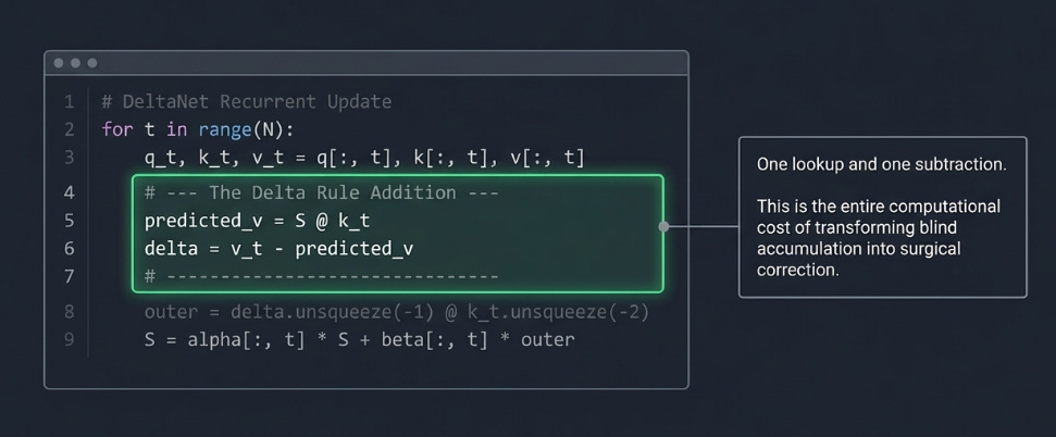
The recurrent form is a small modification to GLA — just three extra lines:
S = torch.zeros(B, H, D, D, device=x.device)
outputs = []

for t in range(N):
    q_t = q[:, t]       # (B, H, D)
    k_t = k[:, t]
    v_t = v[:, t]
    alpha_t = alpha[:, t]
    beta_t  = beta[:, t]

    # Delta Rule: check what S already knows
    predicted_v = torch.einsum(’bhde,bhe->bhd’, S, k_t)
    delta = v_t - predicted_v

    # Forget
    S = alpha_t.unsqueeze(-1) * S

    # Write the correction, not the full value
    outer = delta.unsqueeze(-1) * k_t.unsqueeze(-2)
    S = S + beta_t.unsqueeze(-1) * outer

    # Read
    out_t = torch.einsum(’bhde,bhe->bhd’, S, q_t)
    outputs.append(out_t)
Compare to GLA's loop — the only difference is computing predicted_v and delta before the write. Everything else stays the same. The read step is identical, the forget gate is identical, the outer product structure is identical. One lookup and one subtraction is the entire cost of the Delta Rule.
The Parallelisation Problem
GLA’s recurrence S_t = α_t · S_{t-1} + b_t is a linear function of S_{t-1}. That linearity is what made the parallel prefix scan work — two steps could be algebraically collapsed into one.
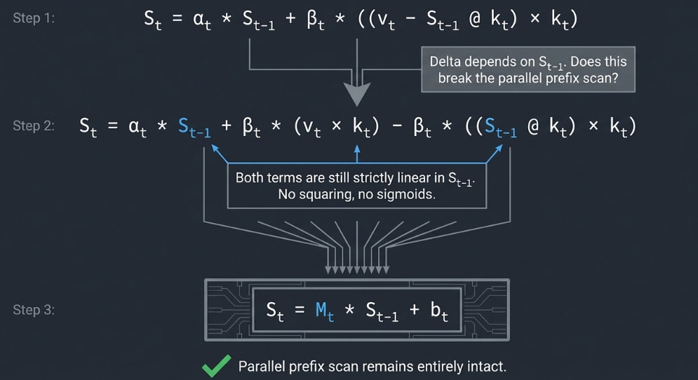
DeltaNet’s update has a wrinkle. The delta depends on the current state:
predicted_v = S_{t-1} @ k_t
delta = v_t - predicted_v
S_t = α_t · S_{t-1} + β_t · (delta ⊗ k_t)
Expand the delta:
S_t = α_t · S_{t-1} + β_t · ((v_t - S_{t-1} @ k_t) ⊗ k_t)
    = α_t · S_{t-1} + β_t · (v_t ⊗ k_t) - β_t · ((S_{t-1} @ k_t) ⊗ k_t)
S_{t-1} appears in two places — once scaled by α, once inside the delta correction. But here’s the key: both terms are still linear in S_{t-1}. There’s no squaring, no sigmoid, no nonlinearity applied to S itself.
This means the recurrence can still be written in the form S_t = M_t · S_{t-1} + b_t, where M_t is a matrix that folds together the forget gate and the delta correction. It’s more complex than GLA’s elementwise α, but it’s still linear — so the parallel prefix scan still applies.
The practical cost is that M_t is a richer transformation than a simple diagonal scale, which makes the fused Triton kernels more involved to write. This is why the FLA library offers both chunk_gla and a separate chunk_delta_rule — same algorithmic idea, but the kernel internals differ.
The Missing Piece: Short Convolutions
There’s a subtle weakness in everything we’ve built so far. The recurrent state S is excellent at tracking global patterns — who the main character is, what the current topic is, facts accumulated over hundreds of tokens. But it’s surprisingly bad at something much simpler: recognizing local phrases.
Think about the phrase “New York City.” Each token enters the recurrence independently — “New” updates S, then “York” updates S, then “City” updates S. At no point does the model see these three tokens together as a unit before they enter the gated update. The outer product v_t ⊗ k_t binds each token’s value to its own key in isolation.
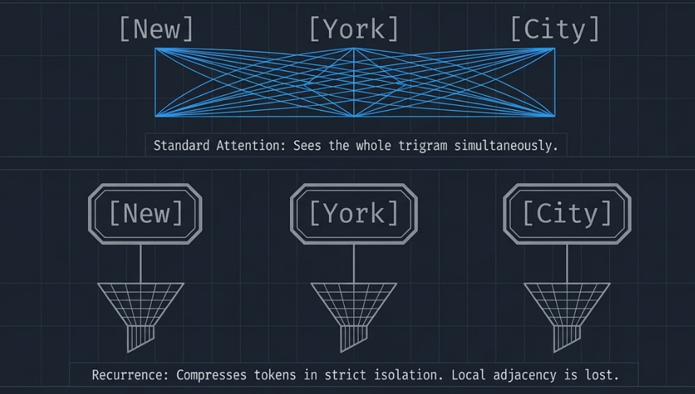
Standard attention doesn’t have this problem. The N×N attention matrix lets “City” directly attend to “New” and “York” in the same operation, naturally capturing the trigram. But our D×D state compresses everything into a fixed-size summary — local adjacency information gets lost in the compression.
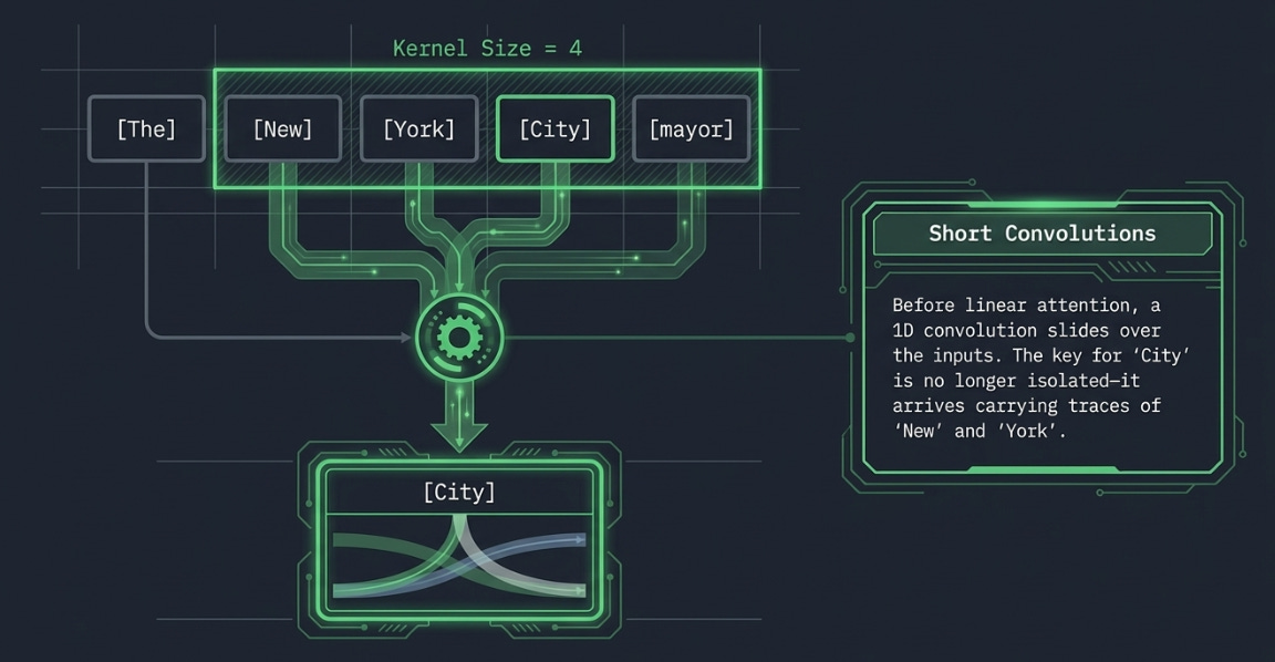
The fix is simple and old: a 1D depthwise convolution applied to Q, K, and V before they enter the linear attention step.
conv(kernel_size=4):  slides a window over the token stream

Input:    [The] [New] [York] [City] [mayor]
                  \_____\_______\______/
Conv output at "City" = weighted mix of {New, York, City, mayor}
A kernel size of 4 means each token gets mixed with its 3 nearest neighbors. After convolution, the key for “City” isn’t just about “City” in isolation — it carries traces of “New” and “York” too. When this enriched key enters the DeltaNet update, the outer product now binds a phrase-aware representation into S rather than a single-word one.
“Depthwise” means each feature dimension is convolved independently — no cross-channel mixing, keeping the operation cheap. The total cost is negligible compared to the linear attention step, but the quality improvement is substantial. This is why virtually every production linear attention model — DeltaNet, Mamba, RWKV — includes a short convolution as standard.
Global memory (DeltaNet) + local context (short conv) = the full picture.
Let’s walk through it concretely.
Say you have 5 tokens, each with a 3-dimensional embedding:
Token 0 "The":   [1, 5, 2]
Token 1 "New":   [3, 1, 4]
Token 2 "York":  [2, 6, 1]
Token 3 "City":  [4, 2, 3]
Token 4 "mayor": [1, 3, 5]
A 1D convolution with kernel size 3 has a small weight vector — one per feature dimension. That’s the “depthwise” part: each dimension gets its own private kernel, no cross-dimension mixing.
Say dimension 0 has kernel weights [0.2, 0.5, 0.3]. To compute the output at token 2 (”York”), the conv slides the kernel over tokens 1, 2, 3:
Dim 0 values at tokens 1,2,3:  [3, 2, 4]
Kernel weights:                 [0.2, 0.5, 0.3]

Output = 0.2×3 + 0.5×2 + 0.3×4 = 0.6 + 1.0 + 1.2 = 2.8
Dimension 1 has its own kernel, say [0.1, 0.7, 0.2]:
Dim 1 values at tokens 1,2,3:  [1, 6, 2]
Output = 0.1×1 + 0.7×6 + 0.2×2 = 0.1 + 4.2 + 0.4 = 4.7
Same for dimension 2 with its own kernel. The output for “York” becomes [2.8, 4.7, ...] — a weighted blend of its neighbors, computed independently per dimension.
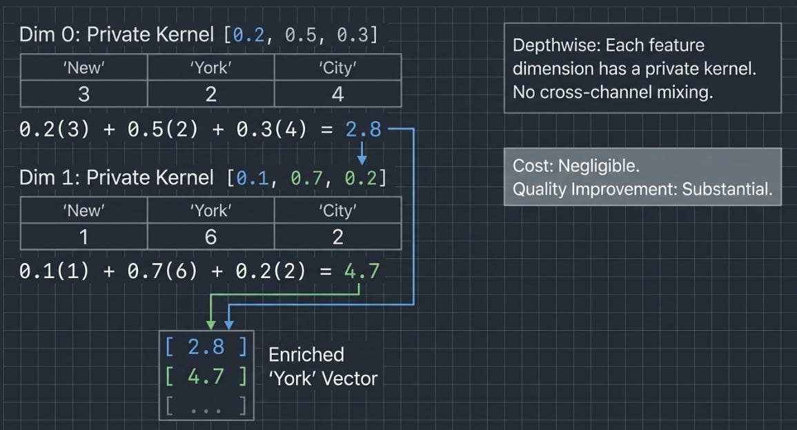
The key insight: after this operation, the representation for “York” now contains information from “New” and “City”. When this enriched vector becomes a key or value in the DeltaNet update, it carries local phrase context that the recurrence alone would miss.
Using FLA’s DeltaNet
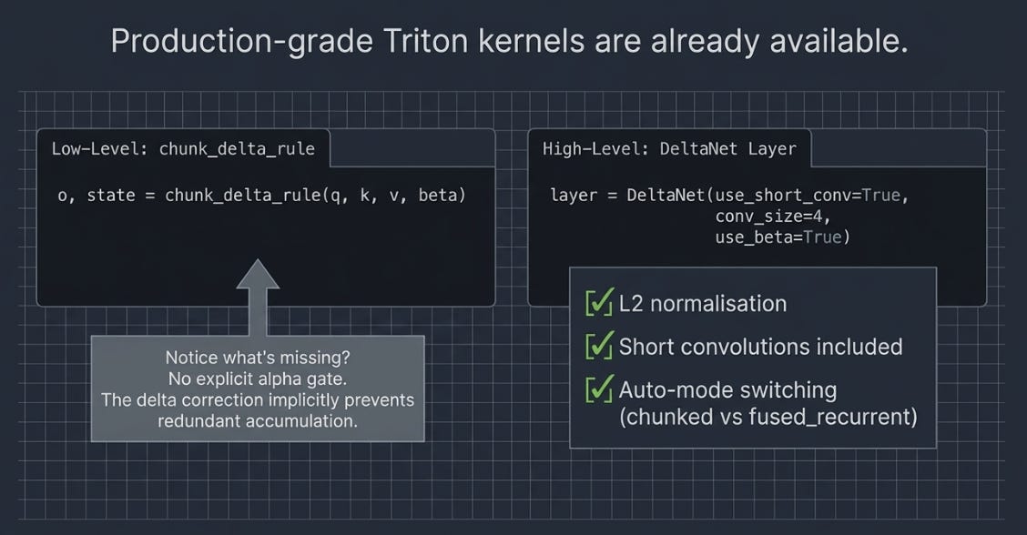
The Flash Linear Attention library provides production-grade Triton kernels for DeltaNet. Like GLA in Part 5, it’s available at two levels.
Low-level kernel — chunk_delta_rule handles the chunked parallel scan directly:
import torch
import torch.nn.functional as F
from fla.ops.delta_rule import chunk_delta_rule

B, T, H, D = 4, 2048, 4, 128
q = torch.randn(B, T, H, D, device=’cuda’)
k = torch.randn(B, T, H, D, device=’cuda’)
v = torch.randn(B, T, H, D, device=’cuda’)
beta = torch.rand(B, T, H, device=’cuda’).sigmoid()

o, final_state = chunk_delta_rule(
    q, k, v, beta,
    initial_state=None,
    output_final_state=True
)
Unlike chunk_gla, there’s no separate α gate. DeltaNet’s delta correction — subtracting what S already knows — implicitly prevents redundant accumulation, reducing the need for an explicit forget gate. The beta gate controls write strength, same as GLA.
High-level layer — drop-in replacement with batteries included:
from fla.layers import DeltaNet

layer = DeltaNet(
    hidden_size=1024,
    num_heads=4,
    use_short_conv=True,
    conv_size=4,
    use_beta=True,
    mode=’chunk’,
).to(’cuda’)

x = torch.randn(2, 2048, 1024, device=’cuda’)
out, _, _ = layer(x)
print(out.shape)    # torch.Size([2, 2048, 1024])
The high-level layer handles the details we’ve discussed — short convolutions on Q, K, V before the attention step, L2 normalisation on queries and keys for numerical stability, and automatic mode switching to fused_recurrent for short sequences where chunking overhead isn’t worth it.
The Full Journey
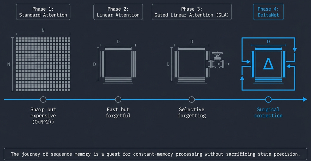
We started this series with a simple matrix multiply — (Q @ K^T) @ V — and the N×N attention map it produces. Six parts later, we’ve arrived at something fundamentally different.
Part 1-2: Standard Attention    → N×N map, sharp but expensive
Part 3-4: Linear Attention      → D×D state, fast but forgetful
Part 5:   GLA                   → + gates, selective forgetting
Part 6:   DeltaNet              → + delta rule, surgical correction
DeltaNet processes sequences in linear time with constant memory, yet maintains a state that can selectively remember, forget, and correct its own knowledge — capabilities that took the RNN field decades to develop, now running at transformer-scale throughput on modern GPUs.
What You Gain, What You Lose
DeltaNet isn’t a free upgrade over standard attention. It’s a different set of trade-offs.
What you gain:
O(N) training cost instead of O(N²) — sequences of 100k+ tokens become practical
Constant inference memory — a fixed D×D state replaces the ever-growing KV cache
Surgical memory management — the delta rule avoids redundant writes and corrects stale information, something even GLA can’t do
What you lose:
Exact token recall — standard attention can pinpoint the exact token where a fact appeared. DeltaNet can only tell you what its compressed state believes. For tasks requiring precise retrieval over long contexts (”what was the third word in paragraph 17?”), this is a real limitation
Proven scaling behaviour — transformers have been scaled to trillions of tokens across hundreds of billions of parameters. DeltaNet and its relatives are younger, with less empirical evidence at the largest scales
Ecosystem maturity — tooling, debugging, interpretability research — all of this is deeper for standard attention
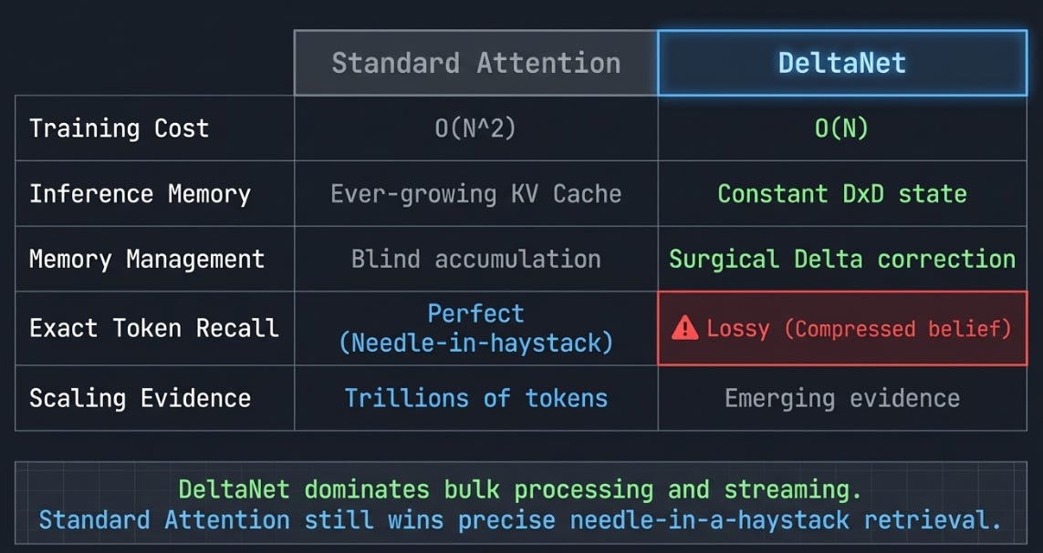
The honest picture: for many practical workloads, especially long-context generation and streaming applications, the trade-off favours DeltaNet. For tasks requiring needle-in-a-haystack retrieval, standard attention still wins. The most promising recent architectures don’t choose one — they hybridise, using linear attention layers for bulk sequence processing and a few standard attention layers where precise recall matters.
What Comes Next
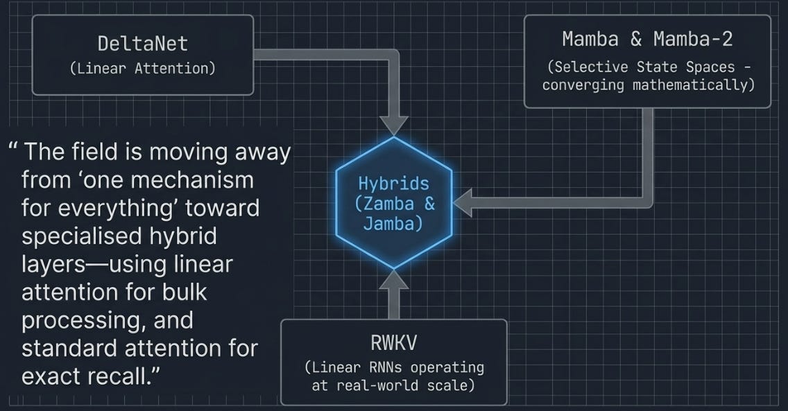
DeltaNet doesn’t exist in isolation. It’s part of a wave of architectures rethinking how sequence models manage memory.
Mamba and Mamba-2 take a different path to the same destination — selective state space models that also achieve linear scaling with data-dependent gating. Mamba-2 in particular drew an explicit connection between state space models and linear attention, showing these two research threads are converging on similar mathematics from different directions.
RWKV pushes the linear RNN idea into production at scale, with open-source models trained on trillions of tokens — providing some of the strongest evidence that these architectures can compete with transformers at real-world scale.
Hybrid architectures are perhaps the most pragmatic development. Rather than picking one approach, models like Zamba and Jamba interleave a few standard attention layers (for precise recall) with many linear attention or SSM layers (for efficient bulk processing). This gets most of the memory savings while preserving the needle-in-a-haystack capability where it matters.
The direction is clear: the field is moving away from “one mechanism for everything” toward specialized layers that each do what they’re best at. DeltaNet and its relatives are a core building block in that future.
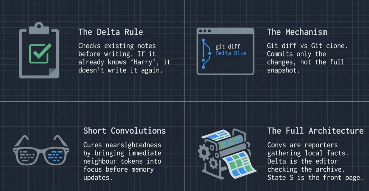
Takeaway Mental Models
DeltaNet is a teacher grading homework. GLA reads your essay and writes notes about it. DeltaNet reads your essay, checks its existing notes first, and only writes down what’s new or corrects what it got wrong. If the notes already say “protagonist is Harry,” it doesn’t write that again.
The delta is a diff, not a snapshot. Think git diff vs git clone. GLA clones the full value into memory every time. DeltaNet computes the diff against what’s already stored and commits only the changes.
Short convolutions are reading glasses. DeltaNet has excellent long-range vision — it can recall facts from thousands of tokens ago. But it’s nearsighted about what’s right in front of it. The short conv is a pair of reading glasses that brings neighbouring tokens into focus before they enter memory.
The full architecture is a newsroom. Short convolutions are reporters on the ground bundling local facts into stories. The delta rule is an editor checking each story against the archive before publishing. The gates decide which old stories to retire and how prominently to run new ones. The state S is the front page — always current, fixed size, lossy but useful.
References
Widrow & Hoff, “Adaptive Switching Circuits” (1960) — the original delta rule for error-driven weight updates
Hochreiter & Schmidhuber, “Long Short-Term Memory” (1997) — gated recurrence for sequence modelling
Katharopoulos et al., “Transformers are RNNs: Fast Autoregressive Transformers with Linear Attention” (2020) — linear attention and the RNN equivalence
Yang et al., “Parallelizing Linear Transformers with the Delta Rule over Sequence Length” (2024) — DeltaNet
Gu & Dao, “Mamba: Linear-Time Sequence Modeling with Selective State Spaces” (2023) — Mamba
Dao & Gu, “Transformers are SSMs” (2024) — Mamba-2 and the connection to linear attention
Flash Linear Attention (FLA) — production Triton kernels
This is Part 6 of the Attention from First Principles series. If you’ve made it this far, you now understand the full arc — from the N×N attention matrix to a constant-memory state that reads, writes, forgets, and self-corrects.
If the series helped you build intuition, a clap or share helps others find it. If something didn’t land or you spotted an error, the comments are open. And if you want to follow along as I explore what comes next — hybrid architectures, hardware-aware kernel design, and scaling these ideas to production — hit subscribe.