

Attention from First Principles - 5
Gated Linear Attention

You’re taking notes while reading a long book.
Every sentence you read, you faithfully write down.
Nothing is ever erased. Nothing is ever revised.At first, this feels safe. You won’t forget anything.
But a few chapters in, something strange happens.
Early assumptions that turned out to be wrong are still in your notes.
Minor details sit next to major plot points with equal weight.
Old context bleeds into new chapters.By the end, your notes do not clarify the story but obscure it.
So you try a different approach.
You start crossing things out.
You highlight what still matters.
You rewrite parts as your understanding evolves.Now your notes feel alive — adapting as the story unfolds.
This raises a question:
If a model is forced to remember everything, how does it avoid drowning in its own memory?
Part 4 of this series ended with a compact D×D memory matrix that replaced the N×N attention map. If you have not read previous part of this series, I will highly recommend you to check that before proceeding here:

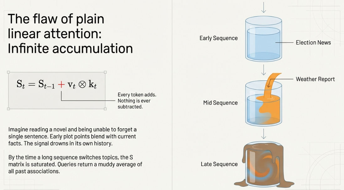
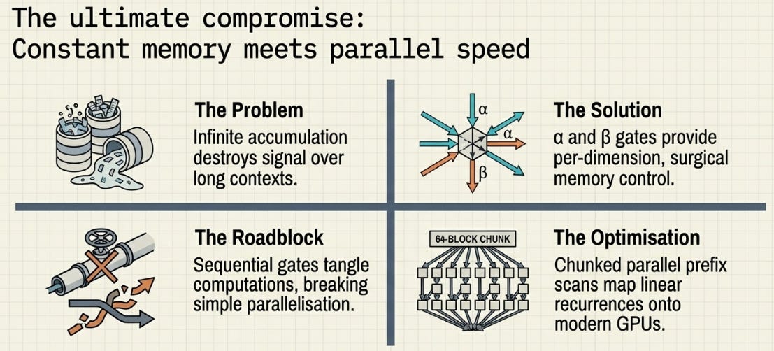
Linear attention gave us constant memory and linear cost — but with a catch. The state S only accumulates. Every token adds to it, nothing is ever removed.
For short sequences, this is fine. For long ones, it’s a problem. Imagine reading a novel and being unable to forget a single sentence. By chapter ten, your notes are a mess — early plot points blending with later ones, outdated facts mixing with current ones. The signal drowns in its own history.
Gated Linear Attention is the fix. It gives the model two learned controls at every token: how much of the old memory to preserve, and how strongly to write the new information. The state S becomes a living thing — selectively forgetting what’s stale and reinforcing what matters.
Where Plain Linear Attention Breaks Down
Recall the recurrent update from Part 4:
S_t = S_{t-1} + v_t ⊗ k_tEvery token adds its key-value association into S. Nothing is ever subtracted. Consider what happens when you process a long document that switches topic midway — say, a news article about elections followed by a weather report.
By the time you reach the weather section, S still contains every political association from the first half. Query it about “forecast” and you’ll get the weather answer contaminated with traces of election results, because those old key-value pairs are still sitting in the matrix. The longer the sequence, the worse this gets — because it has no mechanism to say “that information is no longer relevant.”
This is the accumulation problem. S is a fixed-size matrix trying to hold an ever-growing amount of information. Without some way to manage its contents, it eventually saturates — every query returns the same muddy average regardless of what you ask.
The Circle Closes
If this sounds familiar, it should. RNNs hit this exact wall in the early 1990s. Vanilla RNNs had a hidden state that accumulated information at every step with no control over what stayed and what went. Long sequences caused gradients to vanish or explode, and the hidden state turned into noise.
The fix, when it came, was gating. Hochreiter and Schmidhuber’s LSTM (1997) introduced forget gates and input gates — learned valves that controlled information flow into and out of the hidden state. GRUs (2014) simplified the design but kept the core idea. Gating is what made RNNs actually work on real sequences.
Then transformers arrived in 2017 and sidestepped the whole problem. No hidden state, no accumulation, no gates needed — just attend to everything directly. RNN-style thinking went out of fashion almost overnight.
And now here we are, trying to make transformers efficient enough for long sequences, and the path leads straight back to a hidden state that accumulates information and needs learned gates to manage it. The architecture looks different — a D×D matrix instead of a vector, outer products instead of simple addition, parallel scans instead of sequential loops — but the fundamental challenge is unchanged. A finite memory processing an infinite stream needs to decide what to remember and what to forget.
The difference is that this time around, the gates sit inside a framework that can be parallelized on modern hardware. LSTM’s gates created sequential dependencies that made GPU utilization painful. GLA’s gates are designed from the start to be compatible with the parallel scan algorithms that make training fast.

Two Gates, Two Decisions
GLA replaces the blind accumulation with a gated update:
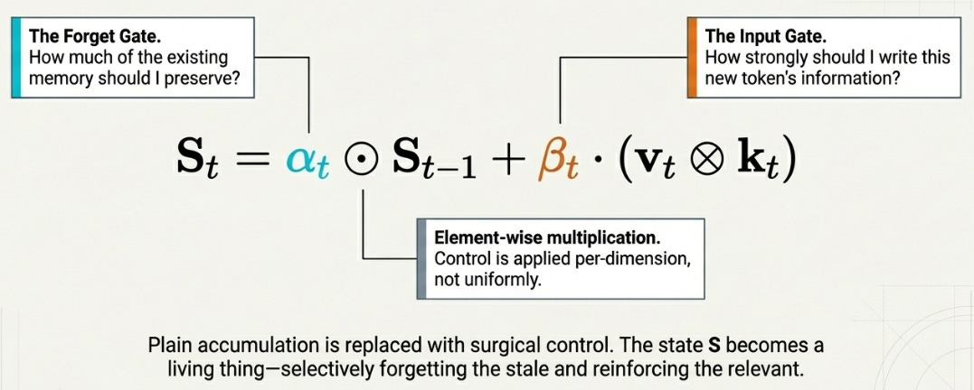
S_t = α_t ⊙ S_{t-1} + β_t · (v_t ⊗ k_t)Two new terms, each making a separate decision at every token.
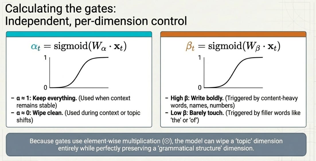
α (the forget gate) answers: “How much of my existing memory should I preserve?” It’s a value between 0 and 1. At α ≈ 1, the old state passes through almost untouched — the model is saying “nothing has changed, keep everything.” At α ≈ 0, the state is nearly wiped clean — “new context, start fresh.”
β (the input gate) answers: “How strongly should I write this new token’s information?” Also between 0 and 1. A content-heavy word like a name or a number gets a high β — write it boldly. A filler word like “the” or “of” gets a low β — barely touch the state.
Both are computed the same way:
α_t = sigmoid(W_α · x_t)
β_t = sigmoid(W_β · x_t)
A learned linear projection of the current token embedding, squashed through sigmoid to land in (0, 1). The model learns from data which tokens should trigger forgetting and which should trigger writing.
The ⊙ in the equation is element-wise multiplication — and this matters. α is not a single number applied uniformly across S. It’s a vector of size D, applying a different forget rate to each dimension. One dimension might track the current topic and need frequent clearing. Another might track grammatical structure and rarely need updating. Per-dimension gating lets the model manage these independently. (Similar is the case with β, it applies, per dimension write)
Gates in Action
Take our familiar D=2 state. After processing a few tokens about elections, S looks like this:
S = [[80, 50],
     [60, 40]]
Now a new token arrives — the start of a weather section. The model produces:
α = [0.1, 0.9]     ← "forget the topic dimension, keep the style dimension"
β = [0.8, 0.3]     ← "write topic strongly, write style weakly"
k = [1, 0]
v = [10, 20]
Apply the update S_new = α ⊙ S_old + β ⊙ (v ⊗ k):
Forget:   α ⊙ S = [[0.1×80, 0.1×50],   = [[ 8,  5],
                    [0.9×60, 0.9×40]]      [54, 36]]

Outer:    v ⊗ k = [[10, 0],
                    [20, 0]]

Write:    β ⊙ (v ⊗ k) = [[0.8×10, 0.8×0],   = [[8, 0],
                           [0.3×20, 0.3×0]]      [6, 0]]

S_new:    [[ 8+8,  5+0],   = [[16,  5],
           [54+6,  36+0]]     [60, 36]]
Look at what happened. The first row — where α was 0.1 — got nearly wiped and overwritten with fresh weather data. The second row — where α was 0.9 — mostly preserved its old values. The model surgically forgot the topic while retaining the style dimension.
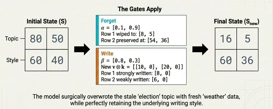
Notice how β works per-dimension too. Dimension 0 (topic) gets written with full force (β=0.8) while dimension 1 (style) gets a gentle touch (β=0.3). Combined with α, the model has independent fine-grained control over both forgetting and writing in every dimension of S.
Parallelizing the Gated Update
In Part 4, we parallelized plain linear attention with cumsum — possible because each token’s contribution was an independent outer product, and cumulative sums are trivially parallel.
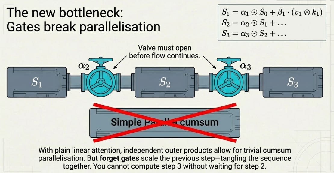
Gates break that. Look at the recurrence again:
S_1 = α_1 ⊙ S_0 + β_1 · (v_1 ⊗ k_1)
S_2 = α_2 ⊙ S_1 + β_2 · (v_2 ⊗ k_2)
S_3 = α_3 ⊙ S_2 + β_3 · (v_3 ⊗ k_3)
Each step depends on the previous S and scales it by a different α. You can’t just cumsum the outer products anymore — the forget gates tangle the steps together.
But the recurrence has a specific structure: it’s linear. Each S_t is a linear function of S_{t-1}. And linear recurrences have a well-known trick for parallelization — the parallel prefix scan.
Why Two Steps Can Become One
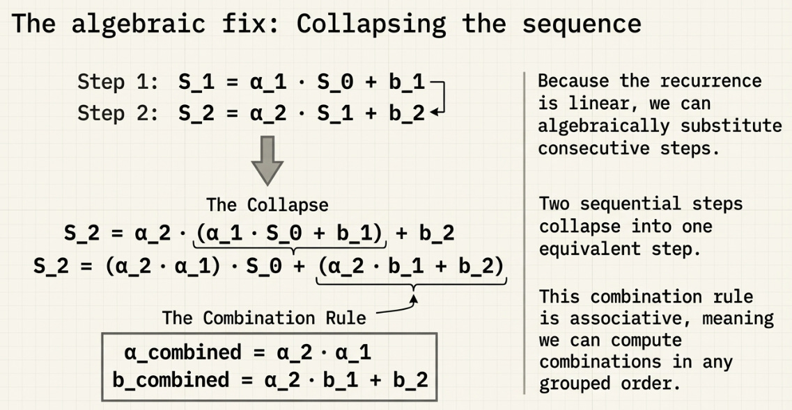
To see how, let’s simplify notation. Write each step as S_t = α_t · S_{t-1} + b_t where b_t = β_t · (v_t ⊗ k_t). Now take two consecutive steps and substitute:
S_1 = α_1 · S_0 + b_1
S_2 = α_2 · S_1 + b_2
Expand S_2 by plugging in S_1:
S_2 = α_2 · (α_1 · S_0 + b_1) + b_2
    = (α_2 · α_1) · S_0 + (α_2 · b_1 + b_2)
Two sequential steps collapse into one equivalent step with:
α_combined = α_2 · α_1
b_combined = α_2 · b_1 + b_2
That’s just algebraic substitution. And because this combination rule is associative — combining (A then B) then C gives the same result as A then (B then C) — we can arrange the combines into a parallel tree.
The Parallel Tree
Take four steps:
Step 1: α=0.5, b=10
Step 2: α=0.8, b=20
Step 3: α=0.3, b=30
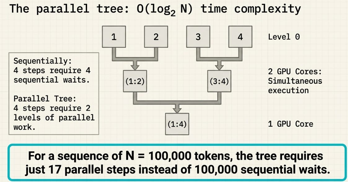
Step 4: α=0.6, b=5Sequentially: step 4 waits for 3, which waits for 2, which waits for 1. Four steps, four waits.
The parallel tree does it in two levels:
Steps:       1       2       3       4
              \     /         \     /
Level 1:     (1:2)            (3:4)       ← 2 cores, simultaneous
                 \             /
Level 2:        (1:2:3:4)                 ← 1 core
Level 1 — two GPU cores work simultaneously:
Core A: combine steps 1 & 2
  α_(1:2) = 0.8 × 0.5       = 0.4
  b_(1:2) = 0.8 × 10 + 20   = 28

Core B: combine steps 3 & 4
  α_(3:4) = 0.6 × 0.3       = 0.18
  b_(3:4) = 0.6 × 30 + 5    = 23
Level 2 — combine the two results:
α_(1:4) = 0.18 × 0.4       = 0.072
b_(1:4) = 0.18 × 28 + 23   = 28.04
Verify against the sequential computation:
S_0 = 0
S_1 = 0.5 × 0 + 10   = 10
S_2 = 0.8 × 10 + 20   = 28
S_3 = 0.3 × 28 + 30   = 38.4
S_4 = 0.6 × 38.4 + 5  = 28.04  ✅
Same answer. Two levels of parallel work instead of four sequential waits. For a sequence of N tokens, the tree has log₂(N) levels — at N = 100,000, that’s 17 parallel steps instead of 100,000 sequential ones.
GLA in Code
Let’s build it up from the recurrent form first, then show the parallel version.
Recurrent mode — clear, readable, slow:
class GatedLinearAttention(nn.Module):
    def __init__(self, d_model, n_heads):
        super().__init__()
        assert d_model % n_heads == 0
        self.n_heads = n_heads
        self.head_dim = d_model // n_heads

        self.q_proj = nn.Linear(d_model, d_model, bias=False)
        self.k_proj = nn.Linear(d_model, d_model, bias=False)
        self.v_proj = nn.Linear(d_model, d_model, bias=False)
        self.alpha_proj = nn.Linear(d_model, d_model, bias=False)
        self.beta_proj = nn.Linear(d_model, d_model, bias=False)
        self.o_proj = nn.Linear(d_model, d_model, bias=False)
        self.norm = nn.GroupNorm(n_heads, d_model)

    def forward(self, x):
        B, N, _ = x.shape
        H, D = self.n_heads, self.head_dim

        q = self.q_proj(x).view(B, N, H, D)
        k = self.k_proj(x).view(B, N, H, D)
        v = self.v_proj(x).view(B, N, H, D)
        alpha = torch.sigmoid(self.alpha_proj(x)).view(B, N, H, D)
        beta  = torch.sigmoid(self.beta_proj(x)).view(B, N, H, D)

        # State S: one (D, D) matrix per batch item per head
        S = torch.zeros(B, H, D, D, device=x.device)
        outputs = []

        for t in range(N):
            # Forget: scale old state per-dimension
            # alpha[:, t] is (B, H, D) — broadcast across last dim of S
            S = alpha[:, t].unsqueeze(-1) * S

            # Write: add gated outer product
            outer = v[:, t].unsqueeze(-1) * k[:, t].unsqueeze(-2)
            S = S + beta[:, t].unsqueeze(-1) * outer

            # Read: query the state
            out_t = torch.einsum(’bhde,bhe->bhd’, S, q[:, t])
            outputs.append(out_t)

        out = torch.stack(outputs, dim=1)            # (B, N, H, D)
        out = out.reshape(B, N, H * D)
        out = self.norm(out.transpose(-1, -2)).transpose(-1, -2)
        return self.o_proj(out)
Five projections from x — the same five we discussed: Q, K, V, α, β. The loop body is three lines that map directly to the equation: forget, write, read.
This runs correctly but the Python loop over N makes it impractical for training. In production, the loop is replaced by a parallel prefix scan implemented as a fused Triton or CUDA kernel — the same tree structure we walked through above, but running on GPU hardware.
Let’s verify it runs:
model = GatedLinearAttention(d_model=64, n_heads=4)
x = torch.randn(2, 128, 64)   # batch=2, seq_len=128, d_model=64
out = model(x)
print(out.shape)               # torch.Size([2, 128, 64])
Same shape in, same shape out — a drop-in replacement for the standard attention layer from Part 1. The difference is entirely internal: instead of an N×N attention matrix, there’s a D×D state matrix that gets selectively forgotten and written at every token.
Production: Beyond the Python Loop
The recurrent implementation above is correct but impractical — a Python loop over 100,000 tokens would take forever. The parallel prefix scan we described fixes the algorithmic problem, but writing a correct and fast GPU kernel for it is non-trivial.
This is where the Flash Linear Attention (FLA) library comes in. Developed by Songlin Yang and collaborators — the same researchers behind the GLA and DeltaNet papers — FLA provides fused Triton kernels that implement the parallel scan on GPU hardware.
But before we see FLA implementation we need to understand one additional concept used for GLA optimization which is Chunking.
Chunking: The Best of Both Worlds
We’ve seen two execution modes — recurrent (sequential, constant memory) and parallel (fast, but materializes all states). Chunking is the practical compromise that production code actually uses.
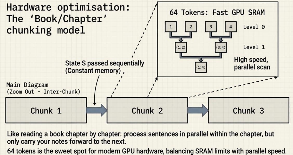
The idea is to split the sequence into fixed-size chunks — typically 64 tokens — and use a different strategy at each level:
Within each chunk — use the parallel form. 64 tokens is small enough that the full computation fits in fast GPU SRAM (the small, ultra-fast memory close to the compute cores). This is where the speed comes from.
Between chunks — pass the final state S forward sequentially. Chunk 2 starts with the final S from Chunk 1. This is where the memory efficiency comes from — only one D×D state needs to be carried forward, not the entire sequence history.
Think of it like reading a book chapter by chapter. Within each chapter, you process all the sentences in parallel. Between chapters, you carry forward your notes.
The chunk size balances two forces. Too small and you don’t get enough parallelism within chunks. Too large and you use too much SRAM. In practice, 64 tokens is the sweet spot for current GPU hardware.
Using FLA in Practice
The Flash Linear Attention library provides production-grade Triton kernels. Here’s how to use GLA at two levels — the low-level kernel and the high-level layer:
Low-level kernel — chunk_gla handles the chunked parallel scan directly:
import torch
import torch.nn.functional as F
from fla.ops.gla import chunk_gla

B, T, H, K, V = 4, 2048, 4, 512, 512
q = torch.randn(B, T, H, K, device=’cuda’)
k = torch.randn(B, T, H, K, device=’cuda’)
v = torch.randn(B, T, H, V, device=’cuda’)
g = F.logsigmoid(torch.randn(B, T, H, K, device=’cuda’))
h0 = torch.randn(B, H, K, V, device=’cuda’, dtype=torch.float32)

o, final_state = chunk_gla(
    q, k, v, g,
    initial_state=h0,
    output_final_state=True
)
Notice two things. First, g is the forget gate in log-space (logsigmoid instead of sigmoid) — this is a numerical stability trick that avoids underflow when multiplying many small gate values together. Second, chunk size isn’t a parameter you set — the kernel automatically picks it (typically 64) based on your sequence length.
High-level layer — drop-in replacement for standard attention:
from fla.layers import GatedLinearAttention

layer = GatedLinearAttention(
    hidden_size=1024,
    num_heads=4,
    mode=’chunk’,
).to(’cuda’)

x = torch.randn(2, 2048, 1024, device=’cuda’)
out, *_ = layer(x)
print(out.shape)    # torch.Size([2, 2048, 1024])
The mode='chunk' (which is the default) uses the chunked parallel scan for training. At inference time, you’d switch to mode='fused_recurrent' for token-by-token generation with constant memory.
Where This Leaves Us
GLA solves the core problem with plain linear attention. The D×D state no longer blindly accumulates — it selectively forgets stale information and controls how strongly new information gets written. Per-dimension gating means different aspects of the state can evolve at different rates, tracking fast-changing context in some dimensions while preserving stable patterns in others.
The parallel prefix scan makes this trainable at scale. Despite being a recurrence — something that historically meant “slow and sequential” — GLA trains as fast as standard attention on modern GPUs, while maintaining the constant-memory inference that makes linear attention attractive in the first place.
But there’s still a gap. GLA’s gates operate blindly — α and β are computed purely from the current token, with no knowledge of what S already contains. The model might write a fact that’s already in memory, or forget a dimension that still holds relevant information, simply because it never checks.
What if, before writing a new key-value pair, the model first asked S: “what do you already know about this key?” And then only wrote the difference — the correction needed, not the full value?
That’s the Delta Rule — and it’s what turns GLA into DeltaNet. Part 6.
References
Hochreiter & Schmidhuber, “Long Short-Term Memory” (1997) — the original LSTM with forget and input gates
Katharopoulos et al., “Transformers are RNNs: Fast Autoregressive Transformers with Linear Attention” (2020) — linear attention and the RNN equivalence
Yang et al., “Gated Linear Attention Transformers with Hardware-Efficient Training” (2023) — GLA, data-dependent gating for linear attention
Yang et al., “Parallelizing Linear Transformers with the Delta Rule over Sequence Length” (2024) — DeltaNet, surgical memory updates
Flash Linear Attention (FLA) — production Triton kernels for GLA, DeltaNet, and related architectures
If this series is helping you build intuition for attention mechanisms, consider subscribing — Part 6 on DeltaNet and the Delta Rule is next, and it’s where the ideas from the last two posts converge into the mountain peak of DeltaNet which powers many of today’s long context models such as the Qwen series LLMs .
If you found this post useful, a clap or share goes a long way in helping others find it. And if something didn’t click or you spotted an error, I’d genuinely like to hear about it in the comments.